When the Cost of Capital Changes Shape
1) The Decision Beneath the Headlines
Many households and investors are not debating rate forecasts. They are making structural choices while uncertainty remains unresolved.
Mortgage terms are being selected. Asset allocations are being adjusted. Cash buffers are being reconsidered. FIRE timelines are being recalibrated.
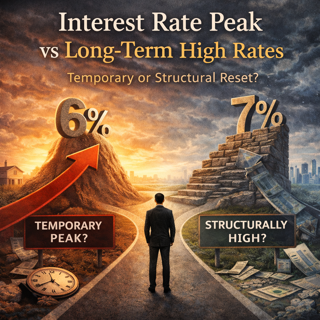
The underlying question is not whether rates rise or fall next quarter. It is whether the current level of interest rates represents a temporary peak or a structural reset higher than the previous decade.
That distinction alters how debt, liquidity, and risk exposure behave over time.
2) Two Plausible Scenarios
Baseline (identical in both cases)
• Household income: $150,000
• Mortgage balance: $600,000
• Investment portfolio: $250,000
• Savings rate: 25% of income
• Time horizon: 10 years
Only one variable changes: the interest-rate path.
Scenario A — Gradual Rate Decline
• Current mortgage rate: 6.5%
• Falls to 4.5% within three years
• Long-term investment returns normalise alongside easing financial conditions
No behavioural change. No additional leverage. Only the rate path differs.
Scenario B — Structural High-Rate Regime
• Mortgage rate remains between 6–7% for the decade
• Borrowing costs stay elevated relative to the prior low-rate era
• Asset valuations adjust to a higher cost of capital
Again, all else remains constant.
3) How the Numbers Diverge
Year 5
Scenario A
Lower mortgage servicing costs free additional cash flow.
Refinancing reduces interest drag.
More capital compounds inside the portfolio.
Scenario B
Higher interest payments persist.
Cash flow remains structurally tighter.
Debt amortisation progresses more slowly.
The difference is not dramatic in year one. By year five, cumulative interest paid meaningfully diverges.
Year 10
Scenario A
Lower servicing costs improve portfolio contribution capacity.
Asset valuations benefit from declining discount rates.
Scenario B
Total interest paid over the decade is substantially higher.
Debt remains a larger share of net worth.
Investment growth must work harder to offset the structural drag.
The divergence is not about return assumptions. It is about how much capital remains available to compound.
Stress Period
Assume a temporary income shock in year seven.
Scenario A
Lower ongoing rate burden allows flexibility.
Liquidity buffers stretch further.
Scenario B
High fixed interest costs compress flexibility.
Liquidity becomes more central than asset valuation.
The stress test does not determine which scenario “wins”. It reveals which structure absorbs shocks more easily.
4) Structural Effects — Not Performance
The difference between these scenarios is not framed in terms of better or worse returns. It is structural.
Cash Flow Stability
Higher long-term rates permanently reduce free cash flow in leveraged households.
Exposure to Timing Risk
Declining rates reward longer-duration assets.
Persistently high rates reward cash discipline and balance-sheet resilience.
Flexibility Under Stress
Lower servicing costs preserve optionality.
Higher servicing costs increase dependency on stable income.
Dependency on Favourable Conditions
Scenario A assumes normalisation.
Scenario B assumes structural repricing.
Each scenario protects against one risk while increasing exposure to another.
5) Hidden Assumptions
For Scenario A to work:
• Inflation moderates sustainably.
• Policy credibility remains intact.
• Economic slowdown does not trigger prolonged stagnation.
For Scenario B to remain viable:
• Income growth keeps pace with higher interest costs.
• Asset prices adjust gradually rather than abruptly.
• Borrowers maintain liquidity buffers.
The visible risk in Scenario A is overconfidence in easing.
The hidden risk in Scenario B is slow erosion of compounding capacity.
6) Long-Term Independence Framing
Financial independence is less about asset returns than about constraint reduction.
A prolonged high-rate regime increases the structural cost of leverage.
A declining-rate regime increases the reward for duration exposure.
The difference influences:
• Savings rate sustainability
• Debt amortisation speed
• Net return assumptions
• Portfolio volatility tolerance
These are precisely the variables stress-tested in the Investment vs Debt Payoff calculator, where interest-rate assumptions and compounding interact directly with cash-flow structure.
The calculator does not predict rates. It clarifies how each rate path reshapes the balance sheet over time.
7) A Grounded Reflection
Interest-rate cycles are often discussed as forecasts. In practice, they are structural forces that shape cash flow and resilience.
If rates fall, leverage becomes less expensive over time.
If rates remain elevated, liquidity and debt discipline become structural priorities.
Neither scenario guarantees advantage. Each rearranges constraints.
Comparison is not about choosing sides. It is about seeing consequences earlier.
Disclaimer: This article is for general information only and is not financial advice. You are responsible for your own financial decisions.

